Correcting Classifier-Free Guidance for Diffusion Models

This work analyzes the fundamental flaw of classifier-free guidance in diffusion models and proposes PostCFG as an alternative, enabling exact sampling and image editing.

NOTE

This work was done as the final project for MIT 6.7960 Deep Learning Course in Fall 2024.

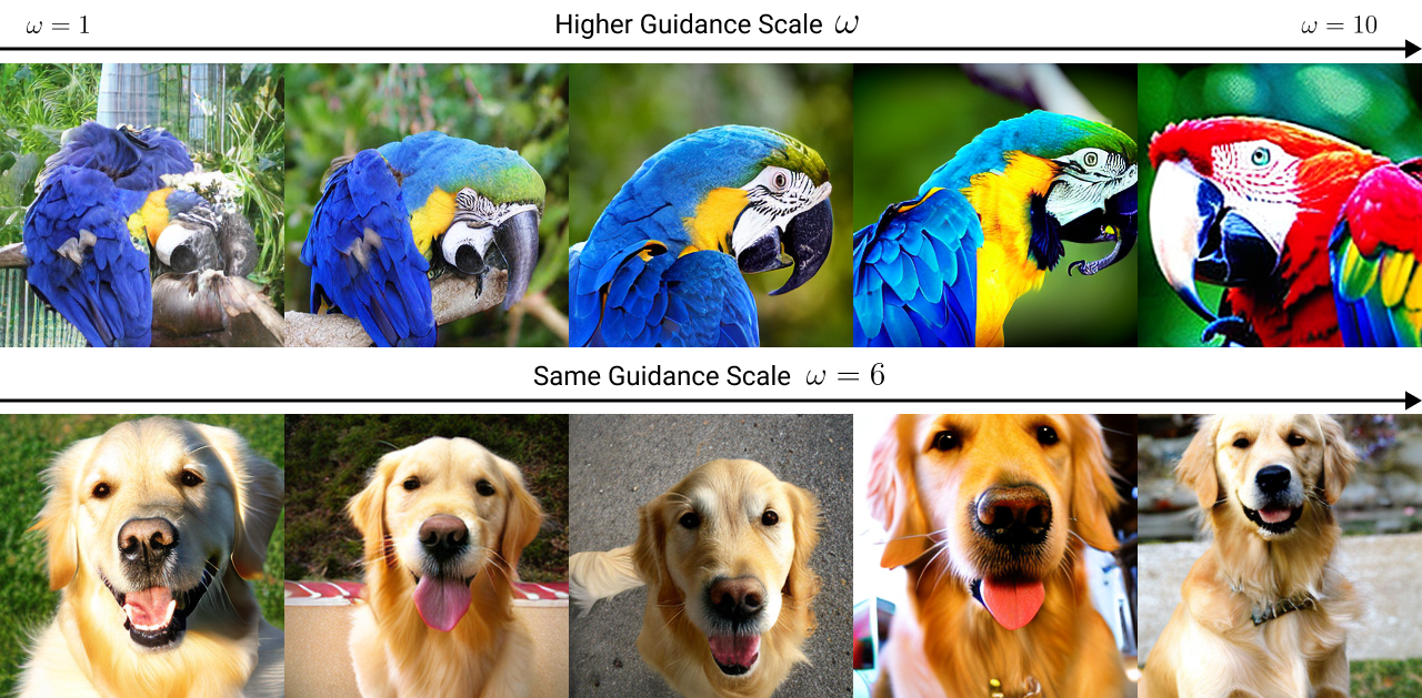
Classifier-free guidance (CFG) is widely used in diffusion models to improve sample quality and alignment with conditions like class labels and text prompts. Despite its benefits, using high guidance scales can lead to problems such as over-saturation, mode dropping, and lack of diversity. This work identifies a fundamental flaw in CFG that causes these problems. We show that CFG’s sampling process is theoretically flawed, even for simple Gaussian distributions, and provide an empirical analysis of how this affects generated samples. Based on this, we propose PostCFG, a novel guidance method that post-processes the samples via Langevin dynamics. Our results on toy Gaussian distributions demonstrate that PostCFG correctly samples from the target distribution, effectively resolving CFG’s issues. Additionally, ImageNet 512x512 and 256x256 experiments show that PostCFG edits samples to better align with conditions, improving sample quality.

Figure 1. PostCFG enables realistic editing of generated images. We present samples of ImageNet at 512x512 and 256x256 resolutions before (top) and after (bottom) applying PostCFG. PostCFG effectively enhances the images by filling in missing details, thereby improving alignment with class labels. Zoom in for a better view.

Introduction

Diffusion models have emerged as a highly expressive and scalable class of generative models, showing remarkable performance on image , video , and audio synthesis tasks. At the core of its success, classifier-free guidance (CFG) has been widely adopted to conditional diffusion models to provide a stronger conditional signal, thereby improving sample quality and conditioning alignment. In practice, high guidance scales are often desired to achieve satisfiable quality and alignment, but it also leads to well-known issues such as over-saturation and mode dropping (See Fig. 2). Several works have proposed to address these issues by reprocessing the guided score function (e.g. by clipping, rescaling, or projecting) , or by applying CFG to only certain intervals of time steps . However, these methods are based on practical heuristics without any theoretical guarantees, and mostly does not generalize well to new tasks or datasets.

In this work, we aim to identify the fundamental cause of these issues in CFG. In particular, we theoretically show that CFG’s sampling process converges to a totally different distribution than the target conditional distribution, even for simple Gaussian distributions. Through empirical analysis, we observe that CFG makes notable errors in sampling at intermediate time steps, leading to highly concentrated samples that lack diversity. Based on these findings, we propose PostCFG that instead post-processes the generated conditional samples via Langevin dynamics. Unlike CFG, PostCFG is guaranteed to sample from the sharpened conditional distribution. Our experiments on toy Gaussian distributions demonstrate PostCFG’s effectiveness in correcting CFG’s issues, converging to the target distribution. Finally, we show that PostCFG successfully edits generated images from ImageNet at 512x512 and 256x256 resolutions, leading to better quality and alignment while maintaining diversity.

Figure 2. Top: Higher guidance scales improve quality but lead to over-saturation & artifacts. Bottom: Samples lack diversity under high guidance scales.

Background

Diffusion Models

Diffusion Models are generative models that learns to reverse the forward diffusion process. The stochastic forward process perturbs a data distribution $p_0(\mathbf{x})$ to $p_T(\mathbf{x}) \approx \mathcal{N}(\mathbf{0}, \mathbf{I})$ by applying a gaussian perturbation iteratively over the time steps $t \in [0, T]$. This can be described by the following stochastic differential equation (SDE) : \begin{equation} \label{eq:sde} d\mathbf{x} = \mathbf{f}(\mathbf{x}, t)dt + g(t)d\mathbf{w} \end{equation} where $\mathbf{f}(\mathbf{x}, t)$ and $g(t)$ are the drift and diffusion coefficients, respectively, and $\mathbf{w}$ is the standard Wiener process. For a time step $t$, the perturbed data distribution is given by $p_t(\mathbf{x})$.

Sampling from the data distribution $p_0(\mathbf{x})$ is achieved by solving either the corresponding reverse SDE (Eq. \ref{eq:reverse-sde}) or the probability flow ordinary differential equation (ODE, Eq. \ref{eq:ode}) :

\begin{equation} \label{eq:reverse-sde} d\mathbf{x} = [\mathbf{f}(\mathbf{x}, t) - \nabla_\mathbf{x} \log p_t(\mathbf{x})]dt + g(t)d\mathbf{w} \end{equation}

\begin{equation} \label{eq:ode} d\mathbf{x} = \left[\mathbf{f}(\mathbf{x}, t) - \frac{1}{2}g(t)^2 \nabla_\mathbf{x} \log p_t(\mathbf{x})\right]dt \end{equation}

Notably, both equations require the score function $\nabla_\mathbf{x} \log p_t(\mathbf{x})$ for every time step $t$, thus a diffusion model is typically trained to estimate this score function or its different parameterization via denoising score matching . We thereby denote a diffusion model as: $ \mathbf{s}_\mathbf{\theta}(\mathbf{x}, t) \approx \nabla_\mathbf{x} \log p_t(\mathbf{x}) $, i.e. a score model that approximates the score function. Existing diffusion samplers are simply discrete solvers of either the reverse SDE stochastic or the probability flow ODE .

Classifier-Free Guidance

Classifier-free guidance (CFG) is introduced by Ho & Salimans for a conditional diffusion model to generate high quality samples by sacrificing diversity. Instead of sampling with a conditional score $\mathbf{s}_\mathbf{\theta}(\mathbf{x}, t, \mathbf{c}) \approx \nabla_\mathbf{x} \log p_t(\mathbf{x} | \mathbf{c})$, CFG samples using the following score estimate: \begin{equation} \label{eq:cfg} \mathbf{s}^{\omega}_\mathbf{\theta}(\mathbf{x}, t, \mathbf{c}) = \mathbf{s}_\mathbf{\theta}(\mathbf{x}, t) + \omega\cdot(\mathbf{s}_\mathbf{\theta}(\mathbf{x}, t, \mathbf{c}) - \mathbf{s}_\mathbf{\theta}(\mathbf{x}, t)) \end{equation} where $\omega \geq 1$ is a guidance scale that pushes the samples towards the mode of the conditional distribution$\omega=1$ corresponds to the original conditional sampling.. Commonly, CFG is implemented by a single diffusion model that can estimate both the unconditional and conditional scores, trained by dropping the condition $\mathbf{c}$ with certain probability. It is a widespread understanding that CFG approximately samples from the sharpened conditional distribution $p^{\omega}(\mathbf{x} | \mathbf{c}) \propto p(\mathbf{x}) \cdot \left(\frac{p(\mathbf{x} | \mathbf{c})}{p(\mathbf{x})}\right)^{\omega}$, which is indeed not the case as we will show in Sec. 3.

Langevin Dynamics

Langevin dynamics enables sampling from a data distribution $p(\mathbf{x})$ using only its score function $\nabla_\mathbf{x} \log p(\mathbf{x})$. Given an initial sample $\mathbf{x} \sim q(\mathbf{x})$ (arbitrary distribution), and a step size $\epsilon$, Langevin dynamics iteratively updates the sample following:

\begin{equation} \label{eq:langevin} \mathbf{x_t} = \mathbf{x_{t-1}} + \frac{\epsilon}{2} \nabla_\mathbf{x} \log p(\mathbf{x_{t-1}}) + \sqrt{\epsilon} \mathbf{w}_t \end{equation} where $\mathbf{w_t} \sim \mathcal{N}(\mathbf{0}, \mathbf{I})$. When $\epsilon \rightarrow 0$ and $T \rightarrow \infty$, Langevin dynamics converges to the target distribution $p(\mathbf{x})$, i.e. $x_T \sim p(\mathbf{x})$. Given a score model $\mathbf{s}_\mathbf{\theta}(\mathbf{x}) \approx \nabla_\mathbf{x} \log p(\mathbf{x})$, Langevin dynamics can be implemented by simply replacing the score function in Eq. \ref{eq:langevin}.

Why is Classifier-Free Guidance Flawed?

Theoretical Analysis

In this section, we revisit the common misconception that CFG approximately samples from the sharpened conditional distribution $p^{\omega}(\mathbf{x} | \mathbf{c})$. Let $p^{\omega}_t(\mathbf{x} | \mathbf{c})$ be a marginal distribution at time step $t$ diffused from the sharpened conditional distribution $p^{\omega}(\mathbf{x} | \mathbf{c})=p^{\omega}_0(\mathbf{x} | \mathbf{c})$ following the forward SDE in Eq. \ref{eq:sde}. To sample from $p^{\omega}$, we need to solve either the reverse SDE or ODE with the score function $\nabla_\mathbf{x} \log p^{\omega}_t(\mathbf{x} | \mathbf{c})$. In CFG, this is replaced by the following: \begin{equation} \label{eq:cfg-score} \mathbf{s}_\mathbf{\theta}^{\omega}(\mathbf{x}, t, \mathbf{c}) \approx \nabla_\mathbf{x} \log p_t(\mathbf{x}) + \omega\cdot(\nabla_\mathbf{x} \log p_t(\mathbf{x} | \mathbf{c}) - \nabla_\mathbf{x} \log p_t(\mathbf{x})) \end{equation}

This is the correct replacement for $t=0$ because $p_0^{\omega}(\mathbf{x} | \mathbf{c}) = p_0(\mathbf{x}) \cdot \left(\frac{p_0(\mathbf{x} | \mathbf{c})}{p_0(\mathbf{x})}\right)^{\omega}$ and

$\nabla_\mathbf{x} \log \left[p_0(\mathbf{x}) \cdot \left(\frac{p_0(\mathbf{x} | \mathbf{c})}{p_0(\mathbf{x})}\right)^\omega\right] = \nabla_\mathbf{x} \log p_0(\mathbf{x}) + \omega\cdot(\nabla_\mathbf{x} \log p_0(\mathbf{x} | \mathbf{c}) - \nabla_\mathbf{x} \log p_0(\mathbf{x}))$, assuming that the score model is well-trained. However, this is not the case for $t>0$ because in general, $ p_t^{\omega}(\mathbf{x} | \mathbf{c}) \propto p_t(\mathbf{x}) \cdot \left(\frac{p_t(\mathbf{x} | \mathbf{c})}{p_t(\mathbf{x})}\right)^{\omega} $ does not hold and thus,

\[\nabla_\mathbf{x} \log p_t^{\omega}(\mathbf{x} | \mathbf{c}) \neq \nabla_\mathbf{x} \log p_t(\mathbf{x}) + \omega\cdot(\nabla_\mathbf{x} \log p_t(\mathbf{x} | \mathbf{c}) - \nabla_\mathbf{x} \log p_t(\mathbf{x}))\]

In fact, this flaw has been acknowledged in previous works , yet, to the best of our knowledge, no work has provided an analysis on the extent of this approximation error and how this error deviates the samples from the target distribution. Now, we analyze these questions through the lens of simple Gaussian distributions.

Why Gaussian Distributions?

To conduct an analysis without making any approximations, we want all distributions and their score functions to be tractable. When conditional and unconditional distributions $p(\cdot | \mathbf{c})$ and $p(\cdot)$ are Gaussian, their noisy versions are also Gaussian, and additionally (noisy) sharpened conditional distributions $p^{\omega}_t(\cdot | \mathbf{c})$ are also Gaussian. Since the score function of a Gaussian distribution is easily computable (linear), all score functions become tractable.

Let $p(\mathbf{x}) = \mathcal{N}(\mathbf{\mu}, \mathbf{\Sigma})$ and $p(\mathbf{x} | \mathbf{c}) = \mathcal{N}(\mathbf{\mu}_c, \mathbf{\Sigma_c})$. For mathematical simplicityNote that this analysis still holds for other types of SDEs, e.g. variance-exploding SDEs., we choose variance-preserving SDE equivalent to: \begin{equation} \mathbf{x}_t = \alpha_t \mathbf{x} + \sigma_t \mathbf{\epsilon} \end{equation} where $\epsilon \sim \mathcal{N}(\mathbf{0}, \mathbf{I})$, and $\alpha_t^2 + \sigma_t^2 = 1$. Then, marginal distributions at time step $t$ are given by:

\[p_t(\mathbf{x}) = \mathcal{N}(\alpha_t \mathbf{\mu}, \alpha_t^2 \mathbf{\Sigma} + \sigma_t^2 \mathbf{I})\] \[p_t(\mathbf{x} | \mathbf{c}) = \mathcal{N}(\alpha_t \mathbf{\mu}_c, \alpha_t^2 \mathbf{\Sigma_c} + \sigma_t^2 \mathbf{I})\]

and the sharpened conditional distribution is $p_t^{\omega}(\mathbf{x} | \mathbf{c}) = \mathcal{N}(\mathbf{\mu}_\omega, \mathbf{\Sigma}_\omega)$ where the following holds:

\[\mathbf{\Sigma_\omega}^{-1} = \omega \mathbf{\Sigma_c}^{-1} + (1-\omega) \mathbf{\Sigma}^{-1}\] \[\mathbf{\Sigma_\omega}^{-1}\mathbf{\mu}_\omega = \omega \mathbf{\Sigma_c}^{-1}\mathbf{\mu}_c + (1-\omega) \mathbf{\Sigma}^{-1}\mathbf{\mu}\]

At time step $t$, the diffused version of the sharpened conditional distribution is given by:

\[p_t^{\omega}(\mathbf{x} | \mathbf{c}) = \mathcal{N}(\alpha_t \mathbf{\mu}_\omega, \alpha_t^2 \mathbf{\Sigma_\omega} + \sigma_t^2 \mathbf{I})\]

Now, let’s see what happens when sampling with CFG. CFG’s score function in Eq. \ref{eq:cfg-score} corresponds to a score function of the following distribution:

\[\tilde{p}_t^{\omega}(\mathbf{x} | \mathbf{c}) \propto p_t(\mathbf{x}) \cdot \left(\frac{p_t(\mathbf{x} | \mathbf{c})}{p_t(\mathbf{x})}\right)^{\omega}\]

and thus, $\tilde{p}_t^{\omega}(\mathbf{x} | \mathbf{c}) = \mathcal{N}(\alpha_t \tilde{\mathbf{\mu}}_\omega, \alpha_t^2 \tilde{\mathbf{\Sigma}}_\omega + \sigma_t^2 \mathbf{I})$ where:

\[\left(\tilde{\mathbf{\Sigma}}_\omega + \frac{\sigma_t^2}{\alpha_t^2} \mathbf{I}\right)^{-1} = \omega \left(\mathbf{\Sigma}_c + \frac{\sigma_t^2}{\alpha_t^2} \mathbf{I}\right)^{-1} + (1-\omega) \left(\mathbf{\Sigma} + \frac{\sigma_t^2}{\alpha_t^2} \mathbf{I}\right)^{-1}\] \[\left(\tilde{\mathbf{\Sigma}}_\omega + \frac{\sigma_t^2}{\alpha_t^2} \mathbf{I}\right)^{-1} \tilde{\mathbf{\mu}}_\omega = \omega \left(\mathbf{\Sigma}_c + \frac{\sigma_t^2}{\alpha_t^2} \mathbf{I}\right)^{-1} \mathbf{\mu}_c + (1-\omega) \left(\mathbf{\Sigma} + \frac{\sigma_t^2}{\alpha_t^2} \mathbf{I}\right)^{-1} \mathbf{\mu}\]

CFG’s sampling process is exact if and only if $\tilde{p}_t = p_t^{\omega}$ for all $t \in [0, T]$. Given that $\tilde{p}_t = p_t^{\omega}$ is equivalent to $\tilde{\mathbf{\mu}}_\omega = \mathbf{\mu}_\omega$ and $\tilde{\mathbf{\Sigma}}_\omega = \mathbf{\Sigma}_\omega$ (try comparing the two equations above!), due to the non-linearity of the inverse operation, this holds only for the two end points: $t=0$ ($\alpha_t=1, \sigma_t=0$) and $t=T$ ($\alpha_t=0, \sigma_t=1$). This indicates that CFG’s sampling process is theoretically flawed for all intermediate time steps, even for simple Gaussian distributions. The update rule using Eq. \ref{eq:cfg-score} deviates from the solution of underlying reverse SDE or ODE, thereby leading to a different distribution.

Empirical Analysis

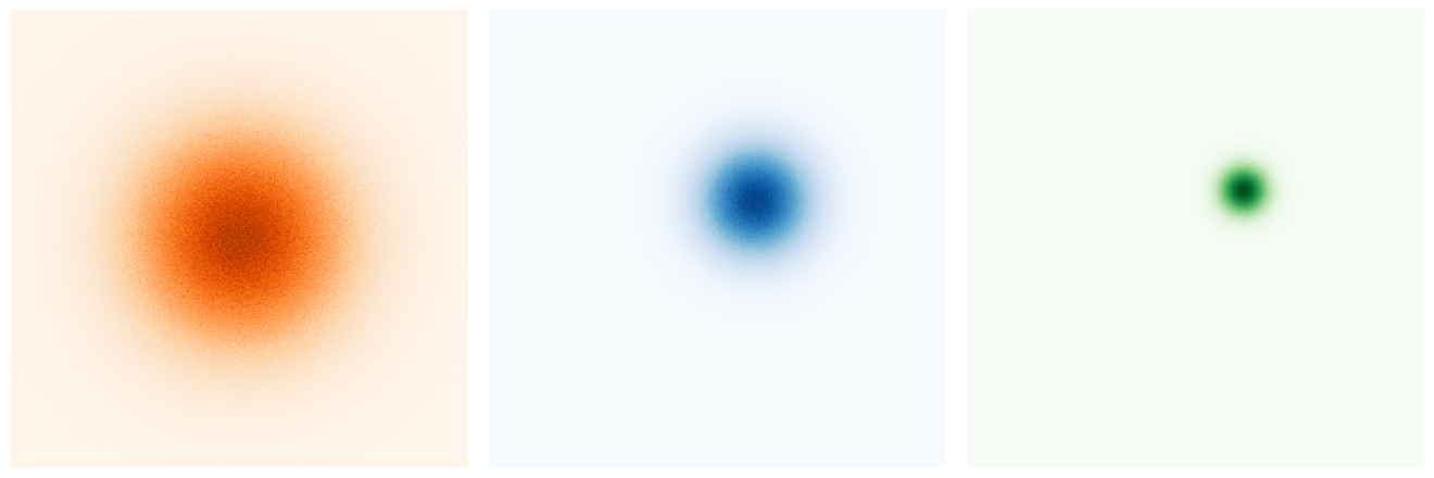
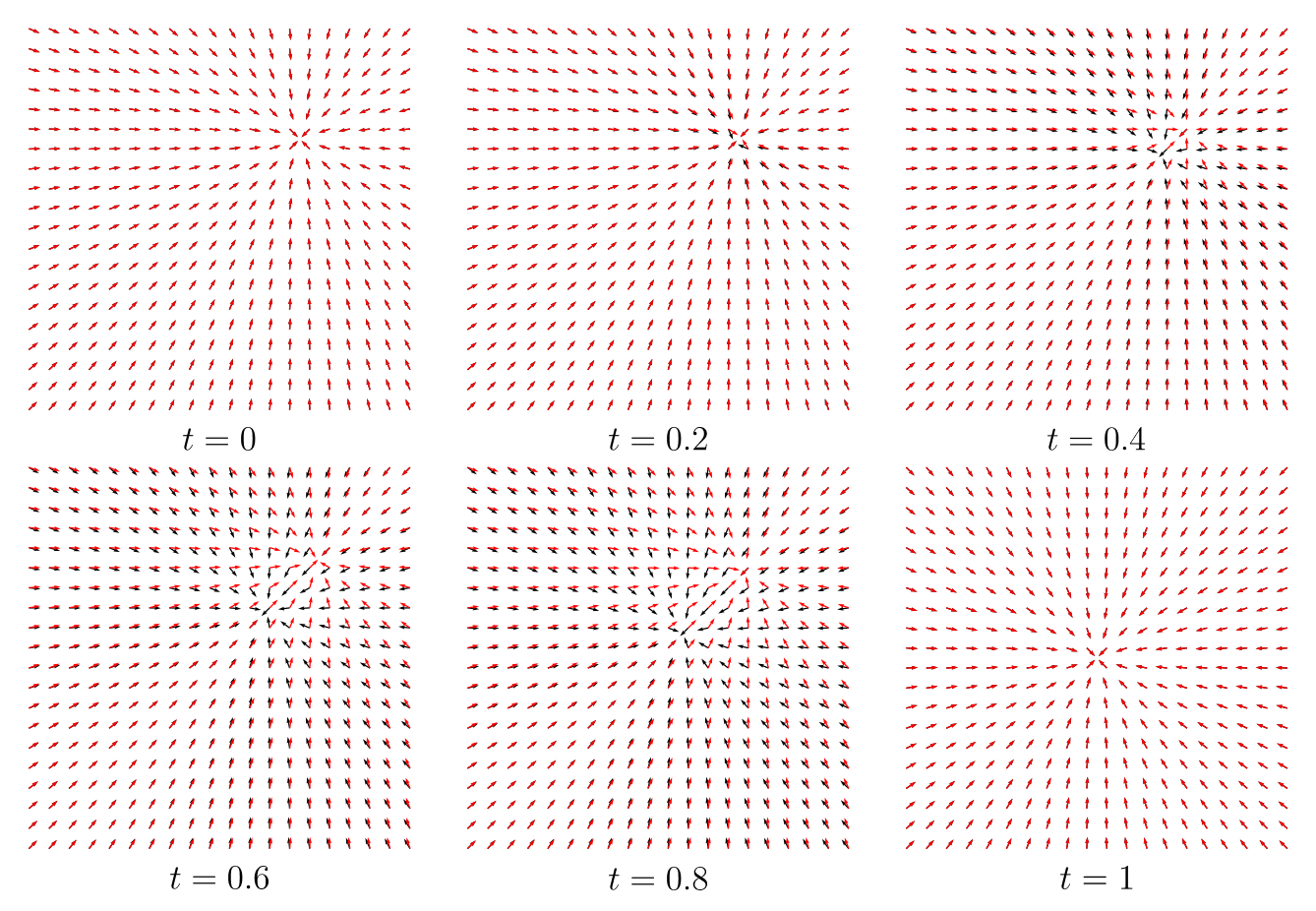
To further analyze the CFG’s sampling process, we present the result of a toy experiment on simple 2D Gaussian distributions in Fig. 3, where $p(\mathbf{x}) = \mathcal{N}((0, 0), \mathbf{I})$ and $p(\mathbf{x} | \mathbf{c}) = \mathcal{N}((0.5, 0.5), 0.5\mathbf{I})$, and $\omega = 6$. As shown in Fig. 4, CFG’s score functions differ from the desired score functions, especially for mid-noise levels ($t = 0.4, 0.6, 0.8$). The result of this error is evident in the generated samples in Fig. 5, where the samples generated by CFG largely deviate from the ground truth samples. Notably, while both DDPM and DDIM samplers lead to mode shifting and smaller variances, DDIM particularly generates highly concentrated samples, probably due to its deterministic nature. These results explain why CFG with high guidance scale leads to over-saturation (= mode shifting) and lack of diversity (= low variance).

Figure 3. Left: Unconditional distribution $p(\mathbf{x})$. Middle: Conditional distribution $p(\mathbf{x} | \mathbf{c})$. Right: Sharpened conditional distribution $p^{\omega}(\mathbf{x} | \mathbf{c})$.

Figure 4. Comparison of exact score functions of $p^{\omega}_t$ and CFG's score functions. Scores are normalized for better visualization.

Figure 5. From left to right: Ground truth samples, Exact (DDPM), Exact (DDIM), CFG (DDPM), CFG (DDIM). Zoomed in around the mode. For each method, we generate 10M samples with 50 sampling time steps.

Method: PostCFG

We propose PostCFG, a novel guidance method that post-processes the generated samples from the conditional distribution $p(\mathbf{x} | \mathbf{c})$ to the sharpened conditional distribution $p^{\omega}(\mathbf{x} | \mathbf{c})$ via Langevin dynamics.

\begin{equation} \bar{\mathbf{x}}_\bar{t} \leftarrow \bar{\mathbf{x}}_{\bar{t}-1} + \frac{\epsilon}{2} \mathbf{s}^{\omega(\bar{t})}_\mathbf{\theta}(\bar{\mathbf{x}}_{\bar{t}-1}, 0, \mathbf{c}) + \sqrt{\epsilon} \mathbf{w}_t \text{ for } \bar{t} \in [1, \ldots, \bar{T}] \end{equation}

where $\mathbf{s}^{\omega(\bar{t})}_\mathbf{\theta}(\mathbf{x}, 0, \mathbf{c})$ is the CFG’s score estimate in Eq. \ref{eq:cfg} for time step $t = 0$, $\mathbf{w}_t \sim \mathcal{N}(\mathbf{0}, \mathbf{I})$, $\epsilon$ is the step size, and $\bar{T}$ is the number of Langevin steps. The Langevin dynamics starts from $\bar{\mathbf{x}}_0 = \mathbf{x}_0 \sim p(\mathbf{x} | \mathbf{c})$ sampled from the conditional distribution using the diffusion model.

Consider a case where $\omega(\bar{t}) = \omega$ for every $\bar{t}$. Then, $\mathbf{s}^{\omega(\bar{t})}_\mathbf{\theta}(\mathbf{x}, 0, \mathbf{c})$ correctly estimates the score function of $p^{\omega}(\mathbf{x} | \mathbf{c})$, and thus, the Langevin dynamics converges to the target distribution $p^{\omega}$ if $\epsilon \rightarrow 0$ and $\bar{T} \rightarrow \infty$. This guarantees that PostCFG correctly samples from the sharpened conditional distribution $p^{\omega}(\mathbf{x} | \mathbf{c})$. In practice, we give a linear dynamic schedule for $\omega(\bar{t})$ following:

\begin{equation} \omega(\bar{t}) = \frac{\bar{t}}{\bar{T}} \cdot \omega \end{equation}

The intuition behind this is that Langevin dynamics suffers from slow mixing when sampling from a multimodal distribution . Thus, it may require many steps with small step sizes to transform the samples from the conditional distribution to the sharpened conditional distribution because the two distributions differ significantly under high guidance scales. By gradually increasing $\omega(\bar{t})$, we can gradually sharpen the marginal distribution, thereby improving the convergence of Langevin dynamics. Note that PostCFG guarantees sampling from the sharpened conditional distribution $p^{\omega}$, even with the dynamic schedule, similarly to annealed langevin dynamics .

Experiments

Revisiting Gaussian

We first revisit the toy experiment on simple 2D Gaussian distributions to demonstrate PostCFG’s effectiveness in correcting CFG’s issues. As shown in Fig. 6, PostCFG successfully generates samples that align with the ground truth samples with 50 Langevin steps. We additionally present a quantitative comparison in Tab. 1, showing that PostCFG significantly outperforms CFG in terms of FID FID is calculated in the same way as in image generation tasks, simply using 2D vectors as features. , and shows a comparable performance to the exact samplers.

Figure 6. PostCFG enables exact sampling from the sharpened conditional distribution. From left to right: Ground truth samples, PostCFG samples with 5, 10, 20, 50 Langevin steps.

Method	Exact (DDIM)	Exact (DDPM)	CFG (DDIM)	CFG (DDPM)	PostCFG (Ours)
FID ($\downarrow$)	0.0003	0.0013	0.1131	0.0180	0.0005

Table 1. FID scores of different methods on the toy Gaussian experiment. PostCFG significantly outperforms CFG.

Image Synthesis

We generate samples from ImageNet at 512x512 and 256x256 resolutions using DiT-XL/2 model, and study the effectiveness of PostCFG.

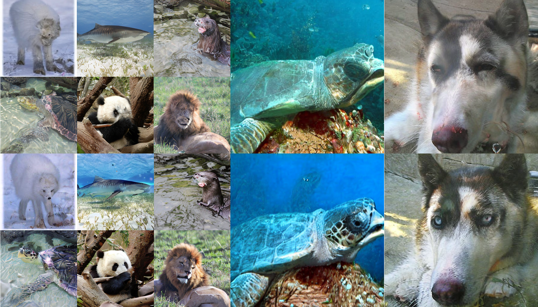
PostCFG enables realistic editing $\;$ Fig. 1 presents the editing capability of PostCFG on class-conditional ImageNet samples. We observe that PostCFG edits the generated images in a realistic manner (e.g. more detailed faces and fur), leading to improved quality and better alignment with class labels. Notably, PostCFG minimally changes the original samples, and thus, in practice, one can use PostCFG to correct the generated images without losing the original style.

PostCFG generates diverse samples $\;$ As shown in Fig. 7, when using a high guidance scale, CFG generates samples that are similar to each other, lacking diversity. In contrast, PostCFG generates more diverse samples. This can be explained in two ways: 1) CFG samples from a distribution that is more concentrated than the sharpened conditional distribution (e.g. Fig. 5), and 2) PostCFG starts from the conditional distribution and only slightly modifies the samples, thereby maintaining diversity.

Figure 7. PostCFG resolves lack of diversity in CFG. Top: CFG. Bottom: PostCFG.

PostCFG reduces over-saturation $\;$ Fig. 8 demonstrates that PostCFG effectively resolves over-saturation in CFG when using high guidance scales. As the guidance scale increases, samples generated by CFG become significantly over-saturated, while PostCFG smoothly gains more details without over-saturation. This can be attributed to the fact that PostCFG samples from the sharpened conditional distribution, whereas CFG samples from another skewed distribution.

Figure 8. PostCFG resolves over-saturation in CFG. Top: CFG. Bottom: PostCFG. Guidance scales increase from left to right: 1, 2, 4, 8, 12.

Limitations

Our work has several limitations. PostCFG often fails to generate realistic samples when the original samples have poor quality, as shown in Fig. 9. This can be attributed to two factors: 1) PostCFG can only modify high-frequency details as Langevin dynamics starts from a clean image. While theoretically Langevin dynamics is independent of the initial distribution, in practice, very many steps are required to modify the low-frequency details. 2) CFG’s superior quality is not solely due to going towards the sharpened conditional distribution. As suggests, CFG effectively removes outliers during the sampling process, leading to better quality. This is not the case for PostCFG as it is post-processing, and this further explains why PostCFG’s visual quality is not as good as CFG, which is another limitation. Finally, we do not provide a quantitative evaluation on ImageNet benchmarks due to compute constraintsFID evaluation requires 50K samples (or at least 1K to be statistically significant)., and thus, we leave this as future work.

Figure 9. Failing cases of PostCFG. Left: Before PostCFG. Right: After PostCFG. PostCFG fails to edit the generated images when the original samples are blurry or lack most details.

Conclusion

We have introduced PostCFG, a guidance method that corrects the fundamental flaw of classifier-free guidance, allowing for exact sampling from the sharpened conditional distribution. PostCFG effectively resolves issues associated with classifier-free guidance, such as over-saturation and limited diversity. Additionally, it brings new post-editing capabilities to diffusion models, which can be leveraged to improve the quality and condition alignment of samples.